Blog

There is no mysticism in amplifier design, just serious science.
—Andrey A. Danilov

Introduction

You will recall from the The Theory of TIM by Matti Otala elsewhere on this site, that one of the consequences of the discovery of TIM in early solid state amplifiers was the erroneous conclusion that it was caused by feedback. By the time high loop gain solid state amplifiers really made their presence felt in the mid 1970’s (remember those Japanese receivers with the cool looking dials and green and blue lights?), vacuum tube amplifiers had ruled the roost for close to 50 years.  The  problem more often than not with tube amplifiers was lack of loop gain, or due to transformer coupling and attendant phase shifts, the inability to apply large amounts to linearize the system – 1% distortion was the norm, but really good designs might get you to the 0.3~0.5% mark at 1 kHz. Reading through solid state technical literature of the time, one comes away with the sense that most designers were groping around in the dark, trying to make sense of the new solid state paradigm, wide bandwidths, high feedback and  how to manage this combination effectively. It is clear with hindsight that although the solutions were ultimately simple, the real cause of the dilemma was that there were a number of interlinking factors, which we will touch on a little later, that took some time to tease apart.

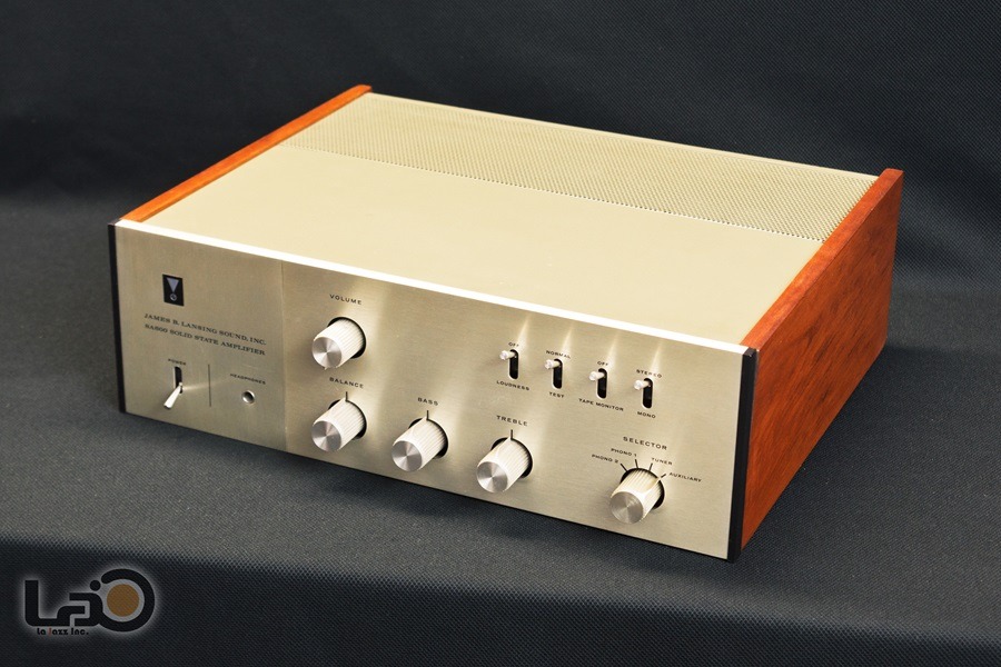
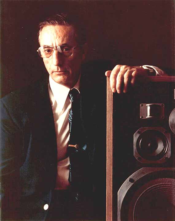
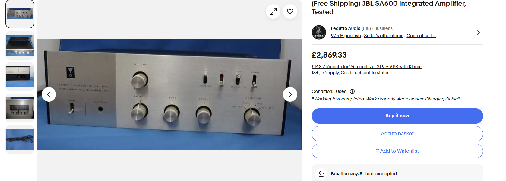
Dealing with the 20 dB loop gains and limited bandwidths that were the norm in tube equipment left the vast majority of designers ill-equipped technically to make the transition to solid state Voltage Feedback Amplifiers  (VFA) where the figures were 40 ~ 50 dB and open loop unity gain loop frequencies of 500 kHz or more. There were a few notable exceptions of course, one of them being Bart Locanthi of JBL who, judging from this design dating from the mid 1960’s was already cognisant of the challenges of high(er) feedback. He employed degeneration of the LTP stage of what was then an early high power solid state amplifier in order to improve the dynamic performance and linearity.  Earlier in his career he had worked in analog computing where much of the research in the 1950’s was around military equipment and  servo systems. He would therefore have been aware of things like loop gain, slewing, transient recovery, phase and gain margin – all critical parameters in servo systems, and as the industry came to learn years later, solid state audio amplifiers, but a rather alien world to vacuum tube consumer electronics designers in the 1960’s.

Prior to Otala’s work, most amplifier designers naively saw feedback as some sort of panacea, to be applied in huge quantities to reduce distortion, invariably quoted at 1 kHz, which masked a host of evils that would be plainly evident at 30 kHz. One could arguably conclude that Otala discovered in TIM what was already known in another engineering discipline (servo and control theory), but  failed to interpret and apply his findings correctly – a point Bruno Putzeys’ touches on in ‘The F Word’.  We owe Otala a debt of gratitude for spurring the industry wide investigation into feedback his paper triggered, but the road to understanding the intricacies of feedback as applied to solid state audio amplifiers, and to being able to build high performance products, was to take at least another twenty years.

The Four Evils

In the first of what I shall term the four evils, many amplifiers from the time ran the front end LTP transistors at very low tail currents in the 1 mA region and I’ve seen power amplifier designs with 500 uA tail currents – so 250 uA in each LTP half. This immediately limited the peak current that could be supplied to the TIS integrator (trans-impedance stage aka VAS), and severely hobbled the LTP’s ability to handle input transients because it lacked the current needed to charge and discharge the compensation capacitor rapidly at HF.  The second evil was the failure to degenerate the LTP transistors – the gm as a result was high, contributing to the high overall loop gain.  Worse however, the high gm results in a narrow linear operating region such that each half of the pair can be ‘flipped’ ON or OFF with very small differential input signals – and that, as we shall see, is a serious shortcoming. The third evil was the lack of high fT, large SOA output devices – the 2N3055/2N2955 and later MJ15003/MJ15004 devices  featured pedestrian 1~2 MHz fT’s – in other words, they were incredibly bandwidth limited and would only work in a system if the unity loop gain frequency (ULGF) was low. All the more reason why Bart Locanthi’s amplifier was such a breakthrough as he built a credible amplifier with what by today’s standards would be seriously compromised output devices.  If one has to try to design an amplifier with these devices today, the unity loop gain frequency would have to be set to 300 kHz – about 5 times lower than in modern amplifiers where  devices like the  NJW3281/1302  are employed that have fT’s of 30 MHz, very high Ic vs hFE linearity and superb SOA capability. This in turn would have then limited the amount of feedback available to correct distortion and is one of the reasons amplifiers from the period generally have distortion figures of 0.007 to 0.01% – about 10x to 15x modern amplifier figures. There were a number of cases where commercial amplifiers would self-destruct if the wrong type of speaker cable was used (it needed to have high inductance to isolate any capacitive load). These products were marginally stable with insufficient gain/phase margin to deal with real world loads.  The fourth evil was that in order to tame the tendency to break into oscillation given the high loop gains and slow output stages, heavy MC (Miller Compensation) around the TIS (VAS) was applied, where I have seen capacitor values as high as 1 nF.  In an attempt to tame the amplifiers predilection to break into oscillation, all sorts of frequency shaping networks were applied across LTP load resistors, or heavy handed shunt compensation was used from the TIS output to ground in these old designs. With modern circuit simulation CAD tools like LTspice, amplifier compensation design and optimization is a cinch – designers in the 1970’s were in effect ‘flying blind’ in this area.

When you present an amplifier with a fast transient on its input,  the LTP pair has to charge the compensation capacitor around the 2nd stage TIS integrator. In an amplifier that suffers from the evils mentioned earlier (and especially evils one, two and four – low tail current, high gm and oversized compensation capacitor), the LTP transistor halves will switch fully ON or fully OFF depending on the signal slope (+ve or -ve). When the amplifier does this, it runs open loop – i.e. without feedback and the output then slews towards one of the supply rails. The result in severe cases is the output rams up against one of the supply rails until the LTP regains control again a few micro seconds later and the loop runs normally again until the next fast music transient. This is what TIM is and it sounded terrible to audiophiles who were used to the smooth, euphonic sound of tubes. In designs that did not go ‘fully TIM’, the amplifier would slew for a shorter period, but not ram up against either of the supply rails. The sound was equally objectionable and this is called SID or Slewing Induced Distortion. There are plenty of commercial amps and DIY designs from the period, that with a full power sine wave stimulus, went into slewing at 30 or 35 kHz  – already absolutely unthinkable by the standards of 1998 when Colloms piece was published.

Superbly Low 1kHz Distortion But Flawed Sonics

With a steady state 1 kHz sine wave input stimulus and near full output power (a typical 1970’s test regime),  a highly compromised amplifier suffering from the 4 evils would test out superbly. How can this be? Amplifier distortion performance  used to be assessed at full power using a 1kHz stimulus.  The output rate of change of a 1 kHz sine wave at the zero crossing on a 100 W amplifier is only about 250 mV per microsecond – a snails pace even for our compromised amplifier, which would pass this test with flying colours, and because of the very high loop gain, distortion would low. Now feed a fast rise time  – say 10 us – 1 kHz square wave stimulus for full output power (about 8 V/us slew rate) and our amplifier performance falls to pieces. Full power square wave testing, or indeed full power HF sine wave testing, was almost never carried out on these products because of cross conduction problems in the output stage – so square wave testing was always small signal – i.e. 1~2 V peak output and the problems alluded to above thus never showed up. Further, testing was usually conducted with a resistive load, so marginally stable designs often slipped through the net and went on to fail in the field because they broke into oscillation with real world capacitive loads.

Otala’s Misguided Legacy: Feedback is Bad

Following Otala’s paper, a number of old wives tales about feedback emerged that still persist despite 40 years of engineering evidence and scholarly research to the contrary – and regrettably repeated in the Colloms article. One enduring fallacy for example, is that the open loop, low corner frequency (a few Hz to maybe a few hundred Hz) that one finds in Miller compensated (MC) amplifiers mean these are ‘slow’ and cannot follow fast music transients and this leads to TIM and the solid state sound.  This is entirely incorrect at every level – the MC open loop corner frequency has nothing to do with slew rate of an amplifier – almost all VFA opamps (other than uncompensated or de-compensated types) use dominant pole (i.e. MC) compensation with corner frequencies of just 1 or 2 Hz that are blindingly fast and even at closed loop gains of 10x or 20x will have -3 dB bandwidths of 3 to 5 MHz,  slew rates of 20 to 50 V/us and full power undistorted rail-to-rail bandwidths of 200kHz. And it is no different with power amplifiers. Slew rate and the open loop bandwidth are set completely independently of each other.

Another fallacy is that feedback is ‘slow’ and there must be a delay around the loop, or that feedback goes multiple times around the loop. Again, on both counts completely incorrect. The loop transit time or loop  ‘flight time’ of a audio power amplifier is about 15 nanoseconds i.e. 0.000000015 seconds to go from the non-inverting input through the amplifying stages to the output and back around via the feedback network to the inverting input. It is not at all dependent on how many stages are involved – 1,2 or 5 its all around the same time give or take a few nano-seconds.  There is therefore no delay in practical terms – only phase shift which is a completely different mechanism and a property of all circuits with reactive components  – with vacuum tube amplifiers exhibiting much greater phase shifts than solid state types. This has nothing to do with the TIM mechanism mentioned above. An amplifier feedback loop is near instantaneous and occurs at relativistic speeds and should not be confused with the slewing in TIM/SID which are entirely down to a combination of  insufficient current to control the TIS compensation capacitor and the high LTP gm.

The feedback ‘doing multiple passes around the loop’ myth grew out of an analysis carried out by Peter J Baxandall  wherein he took a simple single stage amplifier and gradually increased the feedback, monitoring the distortion as he did so. At moderate feedback levels, distortion that was originally less than objectionable 2nd and 3rds folded into higher order harmonics, albeit at lower levels,  that were objectionable. There are a number expositions on this subject (Pass and Boyk and Sussman for example) on the web wherein this phenomena is used to bolster the zero or low feedback argument, but they  use highly compromised, non-linear circuits to try to make their point which is not representative of 21st century SOTA linear amplifier design. These very basic single ended circuits would be seen in hobbyist magazines from the 1950’s and early 1960’s. If you increase the loop gain i.e. feedback, beyond 20 dB, the distortion starts to decrease dramatically, so that at 40 dB loop gain and above, you are getting massive reductions in distortion and it is well below the threshold of human hearing at < 0.01%. The ‘sour’ spot for feedback is indeed the 6 dB to 20 dB region if and only if the amplifier distortion is high in the open loop condition. If it is, either don’t apply any, or make sure you apply plenty as Putzeys points out.  Importantly, the focus on open loop linearity in modern solid state amplifiers means that even with low feedback, they are still superbly linear. Today, we start off with an amplifier that at full power open loop shows much less than 1% THD (good designs are about 0.1%) and we then apply feedback around it – we don’t start with something producing 5%, 10% or 20% which is what Colloms suggests.  Notice also that many of these low feedback/zero feedback designs only quote distortion at low power levels, or at just 1 Watt output. Further, in Pass’ article referenced above, he talks about the problem of IMD in feedback amplifiers. Again, in amplifiers that start off with low open loop distortion, IMD is a non-issue – in modern designs -100 dB down on the test tones which are at full power. Zero and low feedback amplifiers cannot match this performance.

Amplifier Feedback: Figuring it All Out

It took until the mid-1980’s for engineers to figure out what was going on  – although people like Bob Cordell and Bob Sickler were years ahead of the general industry curve –  and another few years for this to percolate through the design community so that only by the early 1990’s do really capable solid state amplifiers that address all of the shortcomings outlined above, become the norm. Alas, those that bought into the idea that feedback was bad, ended up corrupting the whole science of amplifier design for  large parts of the audio amplifier design community, and the press,  and a sub-culture of subjectivism emerged wherein sub-standard products – in every sense of the word – are feted as ‘jaw dropingly good’ or ‘providing fundamentally new insights’ into music never before experienced.  Reality says it’s an amplifier and simply needs to have zero distortion, zero TIM and drive any speaker load down to 2 Ohms with better than 0.2 dB flatness from 20 Hz to 20 kHz. Insofar as slew rates are concerned, the minimum figure acceptable in modern amplifiers is 1 V/us per peak output volt. Thankfully in 2017 all of these requirements are fully realizable at reasonable cost (figure on $30-$35 per stereo watt 2017 retail price on a high end class AB amplifier). In the semiconductor industry, no feedback qualms exist, and hundreds of millions of opamps working in end customer feedback loops are sold and applied every year and work flawlessly – including the ones present in the output stages of every high performance Audio DAC on the market.

Ensuring amplifiers (and specifically VFA types) don’t suffer excessive distortion nowadays is straightforward  because the associated mechanisms are fully and completely understood. And, in 2017 we really do understand the intricacies of negative feedback as applied to audio amplifiers, which it turns out in the big scheme of things, is an exceedingly simple application of control theory science. Firstly, make the amplifier linear in the open loop condition. This is easy to do and a well designed exemplar will be well below 1% at full power open loop i.e. zero feedback and nothing like the 20% Martin Colloms mentions which is the kind of open loop distortion one would expect to see in a sub-par tube amp. Secondly, ensure the LTP is degenerated so that under a worst case full scale input transient with fast rise times (1-2 us), it still operates in the linear portion of its transfer curve and does not approach cut-off.  In most cases this will necessitate some bandwidth limiting of the input signal but in high performance designs, this will be at 300+ kHz. Third, run the front end LTP stage ‘rich’ – i.e. at a high tail current.  Combined with the degeneration this will provide a large linear operating region of 1~1.5 Volts resulting in very low open loop distortion of the LTP; the high tail current means large transient currents can be supplied into and out of the TIS integrator stage. The result is no chance of TIM ever arising. Separately, the LTP must also be well balanced – a point Self stresses in Audio Power Amplifier Design.  Fourth, use modern, high fT, sustained beta output devices like the MJL1302/1381. Finally, close the global feedback loop such that there is a minimum of 45 degrees phase margin at the unity loop gain frequency – typically about 1.5 MHz in modern amplifiers employing EF3 output stages and higher than this in EF2’s. This is not an exhaustive list –  see Douglas Self and Bob Cordell’s books on amplifier design for a more in-depth treatment of the subject.

The Zero TIM Amplifier

Current Feedback Amplifiers  (CFA) first became available in IC form in the early 1980’s. Their prime application in the IC realm was (and still is) in very wideband, high speed  amplifiers – video drivers, telephony systems and test and measurement gear. Their operation is not as intuitive as VFA’s and they really have only come into more widespread use in audio power amplifiers the last 10 or 15 years. Had they been around in the 1960’s, it is arguable that most of the problems discussed in the preceding paragraphs would not have arisen – perhaps only compensation design and that is a relatively easy problem to get ones head around. Matti Otala would never written about the solid state amplifier sound or TIM, and the ‘solid state’ sound would have been a thing of wonder, and not a derogatory remark hurled at some highly compromised amplifier.  Why would this have been the case? CFA’s cannot  produce TIM since the front end quiescent current is not fixed as it is in VFA’s  – it is directly related to the output voltage and the value of the feedback resistor so it is expansive, and not compressive, providing current on demand to charge the compensation capacitor – typically up to 8x the standing value in a practical audio amplifier.  It is not possible to get a CFA’s to slew rate limit  – something even modern VFA’s will do when the LTP runs out of steam at 150~300 kHz (this is 5~10x the figure one would encounter in a mid 1970’s amplifier by the way).  With modern output devices, CFA  power amplifiers are quite capable of reproducing a very credible 100 kHz square wave at full output power into an 8 ohm load – see  the Ovation nx-Amplifier write up for example, page 14.  Lets also be clear here, modern VFA amplifiers that apply the cures for ‘The Four Evils’ discussed above will never go into slew rate limiting with music signals – the TIM problem  that plagued this topology in the 1970’s and early 1980’s is long gone – the issue is completely and wholly solved.

 Sighted Evaluation and Subjectivism

Studies have shown that  human auditory memory is extremely fickle. We are designed to remember the information (who, what, where etc) encoded in sounds and speech, and much less so the exact details of the frequency, harmonic content, precise timing and so forth (note that this is not the same thing as remembering or being able to play a tune or sing in tune which is covered in the cognitive neuroscience of music). Double blind and ABX tests make this abundantly clear where most individuals struggle to tell the difference between amplifiers producing 0.5% distortion and those producing only a fraction of that. Further, we may be able to tell that there is a difference on switching from one to the other, but 5 or ten minutes later, assuming the differences are not gross – which they never are anyway – the chances of a correct identification are indeed slim, and research suggests short term auditory memory of the type being discussed here is about 10 seconds. We do also know that people find higher order harmonics objectionable and lower orders (2nds and 3rds particularly) euphonic. What science also tells us is that when it comes to hearing, like sight, as a species we are susceptible to inference – we believe what is suggested or inferred we heard because we have been told, or because A looks better than B. Therefore, claims that amplifier x is better than y based on sighted testing should always be questioned.  If you want to get to the truth of an amplifier comparison, there is no other way than the scientific way and that means DBT or ABX test methodology. Now, none of this means a thing if someone’s prime motivation for buying a piece of equipment is for looks, bling factor, bragging rights or some other subjective criteria – but then we are not talking about accurate sound reproduction, but about fashion.

The Golden Age of Audio

Today, in both professional and consumer markets, and in the DIY community, you can find solid state feedback amplifiers featuring distortion levels of <10 parts per million at 20 kHz, slew rates of 200 V/us or more along with the ability to drive enormously difficult, reactive loads. None of these amplifiers – VFA or CFA – have a hint of TIM, SID or any other kind of distortion – they are as close as it comes to a piece of wire with gain – Peter Walker’s famous aphorism.  Over the last decade or so, newer, more in-depth understanding of the way humans perceive distortion has emerged. We know, based on research that simple THD and IMD distortion metrics may not tell us the whole truth about what kind of non-linearity we can tolerate when we listen to  a piece of music. However, it is my contention (and Douglas Self no doubt would agree) that a modern, well engineered amplifier’s distortion profile (THD, IMD, GedLee, Rnonlin etc) is orders of magnitude below the hearing threshold. There is no distortion and the amplifier is effectively ‘blameless’.  I know from my experience with a high resolution system that it is very easy to pick out CD’s and LP’s in which clipping and other distortion artefacts can be discerned that have arisen in the recording chain that in all likelihood would not be audible on a legacy system – be it solid state or tube based. We are truly living in the golden age of amplification – and it has everything to do with a thorough and in-depth understanding of feedback and compensation design at an engineering level and all of the mechanisms of non-linearity in the amplifier.

How do these modern, well engineered audio amplifiers sound? Open, effortless, smooth, detailed and supremely accurate – sound quality and performance that could only be dreamt of 40 years ago.